代码:
setwd("D:/Desktop/0000/R") #更改路径

#导入数据
df <- read.table("Input data.csv", header = T, sep = ",")

# -----------------------------------
#所需的包:
packages <- c("ggplot2", "tidyr", "dplyr", "readr", "ggrepel", "cowplot", "factoextra")
#安装你尚未安装的R包
installed_packages <- packages %in% rownames(installed.packages())
if (any(installed_packages == FALSE)) {
  install.packages(packages[!installed_packages])
}
invisible(lapply(packages, library, character.only = TRUE))

# -----------------------------------
# 设置一些颜色、文字的基础设置
# Colors:
CatCol <- c(
  CSH = "#586158", DBF = "#C46B39", EBF = "#4DD8C0", ENF = "#3885AB", GRA = "#9C4DC4",
  MF = "#C4AA4D", OSH = "#443396", SAV = "#CC99CC", WET = "#88C44D", WSA = "#AB3232"
)
Three_colorblind <- c("#A8AD6F", "#AD6FA8", "#6FA8AD") #c("#809844", "#4f85b0", "#b07495")
graph_elements_dark <- "black"
plot_elements_light <- "gray75"
plot_elements_dark <- "gray25"

# Transparency:
boot_alpha_main <- 0.9
boot_alpha_small <- 0.05

# Text:
# if (n_pcs > 3) {x_angle <- 270; x_adjust <- 0.25} else {x_angle <- 0; x_adjust <- 0} # option to change orientation of x axis text
x_angle <- 0; x_adjust <- 0
title_text <- 9 # Nature Communications: max 7 pt; cowplot multiplier: 1/1.618; 7 pt : 1/1.618 = x pt : 1; x = 7 / 1/1.618; x = 11.326 (round up to integer)
subtitle_text <- 9
normal_text <- 9 # Nature Communications: min 5 pt; cowplot multiplier: 1/1.618; 5 pt : 1/1.618 = x pt : 1; x = 5 / 1/1.618; x = 8.09 (round up to integer)

# Element dimensions:
plot_linewidth <- 0.33
point_shape <- 18
point_size <- 1.5

# Initialize figure lists:
p_biplot <- list(); p_r2 <- list(); p_load <- list(); p_contr <- list(); col_ii <- list()

# Labels:
veg_sub_labels <- c("All Sites", "All Forests", "Evergreen Needle-Forests")

# -----------------------------------
#选择PCA所需的数据
codes_4_PCA <- c("SITE_ID", "IGBP", "GPPsat", "wLL", "wNmass", "wLMA", "RECOmax")
#执行筛选
df_subset <- df %>%
  dplyr::select(all_of(codes_4_PCA))
#运行PCA
pca_result <- FactoMineR::PCA(df_subset %>% dplyr::select(-SITE_ID, -IGBP), scale.unit = T, ncp = 10, graph = F)

# -----------------------------------
#绘图
p1<- fviz_pca_biplot(pca_result,
                     axes = c(1, 2),
                     col.ind = df_subset$IGBP, #"grey50",
                     # col.ind = NA, #plot_elements_light, #"white",
                     geom.ind = "point",
                     palette = CatCol,#'futurama',
                     label = "var",
                     col.var = plot_elements_dark,
                     labelsize = 3,
                     repel = TRUE,
                     pointshape = 16,
                     pointsize = 2,
                     alpha.ind = 0.67,
                     arrowsize = 0.5)

# -----------------------------------
# 它是ggplot2对象,我们在此基础上进一步修改一下标注。
p1<-p1+
  labs(title = "",
       x = "PC1",
       y = "PC2",
       fill = "IGBP") +
  guides(fill = guide_legend(title = "")) +
  theme(title = element_blank(),
        text = element_text(size = normal_text),
        axis.line = element_blank(),
        axis.ticks = element_blank(),
        axis.title = element_text(size = title_text, face = "bold"),
        axis.text = element_text(size = normal_text),
        #plot.margin = unit(c(0, 0, 0, 0), "cm"),
        # legend.position = "none"
        legend.text = element_text(size = subtitle_text),
        legend.key.height = unit(5, "mm"),
        legend.key.width = unit(2, "mm")
  )
p1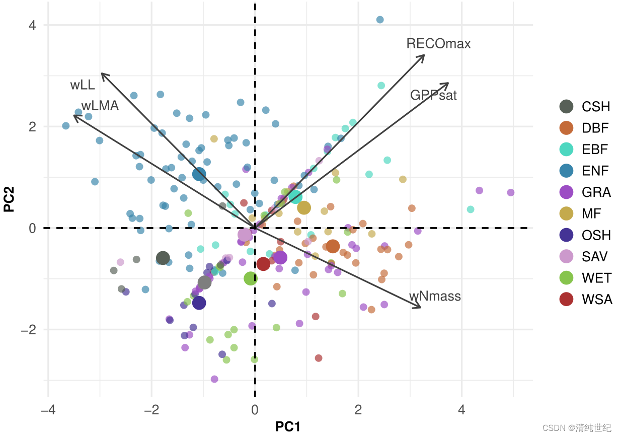
数据:PCA双标图、碎石图R代码、数据.zip - 蓝奏云