单向RNN
这几天一直在看RNN方面的知识,其中最感到疑惑的是下面的两张图。下面两张图说出了单向循环神经网络的所有原理,但是这里面其实是有一点问题的。比如下面第一张图,整个RNN的构成其实是有三个矩阵的。首先输入向量通过输入矩阵U,与上一个的隐藏层状态乘以权重矩阵W后相乘得到了这一层的隐藏状态ht,ht通过权重矩阵V得到最后的输出。
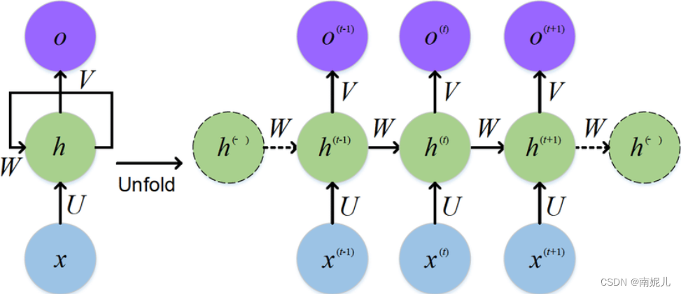
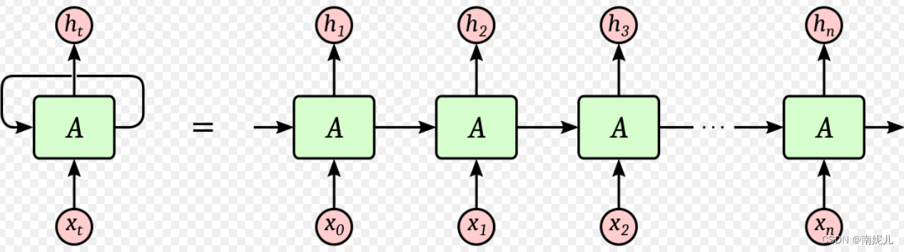
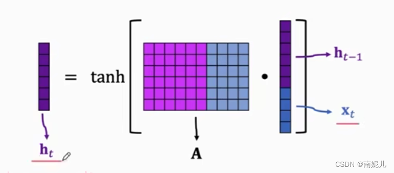
下面这一张图更加简单,整个RNN共用一个矩阵。下图的第二张图讲的非常清楚。将上一层的隐藏层状态和当前的输入拼接送入权重矩阵A中得到本层的隐藏层的状态。
pytorch中 RNN的实现
RNN — PyTorch 1.13 documentation

上面是隐藏层的的计算公式。这也说明了RNN为什么叫做循环神经网络,因为它是不同时序的数据共用一个权重矩阵。
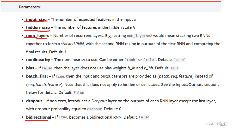
结合一下下面这张图解释一些RNN中参数的含义。
input_size:表示 输入特征的维度。也就是x0的维度
hidden_size:表示隐藏层的输出维度。也就是h1的维度
num_layers: 表示中间隐藏层的个数。上图表示只有一个隐藏层,也就是只有一个权重矩阵A
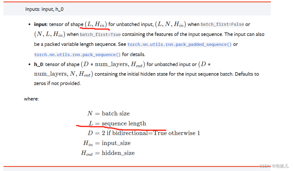
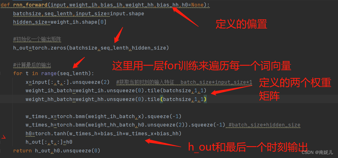
seq_lenth : 表示词向量的个数。就是上图中x0,x1,x2这些向量的个数。这里解释一下计算的过程,首先x0输入RNN网络中,得到隐藏层的状态,隐藏层的状态被保留了下来,然后输入下一个向量,这时添加上一个时刻的隐藏层的状态,可以得到之前的信息。下面的代码可以看出有个for循环,就是遍历每一个词向量。最后的输出包含两个变量,一个是所有时刻输出组成的向量,一个是最后一个时刻的输出。一般使用最后一个时刻的向量就可以,因为这个向量就已经包含了前面所有的信息。
bidirectional:表示的是是否使用双向的RNN。
import torch
import torch.nn as nn

batchsize=2
seq_lenth=3   ##时间长度
input_size=10
hidden_size=5

#随机初始化一个随机序列
input=torch.randn(batchsize,seq_lenth,input_size)
#随机一个初始状态
h0=torch.zeros(batchsize,hidden_size)

#setp1 调用pytorch中API
signal_rnn=nn.RNN(input_size=input_size,hidden_size=hidden_size,batch_first=True)
rnn_output,hn=signal_rnn(input,h0.unsqueeze(0))

# print('所有的隐藏层输出',rnn_output.shape)
# print('最后一个隐藏层的输出',hn.shape)
print('RNN的输出')
# print('所有的隐藏层输出',rnn_output)
print('最后一个隐藏层的输出',hn)
print('最后一个时刻RNN的输出',rnn_output[:,-1,])

#step2 自己手写实现简单的API
def rnn_forward(input,weight_ih,bias_ih,weight_hh,bias_hh,h0=None):
    batchsize,seq_lenth,input_size=input.shape
    hidden_size=weight_ih.shape[0]

    #初始化一个输出矩阵
    h_out=torch.zeros(batchsize,seq_lenth,hidden_size)

    #计算最后的输出
    for t in range(seq_lenth):
        x=input[:,t,:].unsqueeze(2)  #获取当前时刻的输入特征  batch_size*input_size*1
        weight_ih_batch=weight_ih.unsqueeze(0).tile(batchsize,1,1)
        weight_hh_batch=weight_hh.unsqueeze(0).tile(batchsize,1,1)

        w_times_x=torch.bmm(weight_ih_batch,x).squeeze(-1)
        w_times_h=torch.bmm(weight_hh_batch,h0.unsqueeze(2)).squeeze(-1) #batch_size*hidden_size
        h0=torch.tanh(w_times_h+bias_ih+w_times_x+bias_hh)
        h_out[:,t,:]=h0
    return h_out,h0.unsqueeze(0)

#验证一下rnn_forward的正确性
# for pram,name in signal_rnn.named_parameters():
#     print('参数',pram,'值',name)

custom_rnn_output,custom_state_final=rnn_forward(input,signal_rnn.weight_ih_l0,signal_rnn.bias_ih_l0,signal_rnn.weight_hh_l0,signal_rnn.bias_hh_l0,h0=h0)

print('单向RNN')
# print(custom_rnn_output)
print('单向RNN的最后输出',custom_state_final)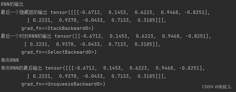
讲到这里差不多就明白了RNN的基本知识了。
RNN实战
import numpy as np
import matplotlib.pyplot as plt

# 生成一些数据,并且可视化
steps = np.linspace(0, np.pi*4, 100, dtype=np.float)
x_np = np.sin(steps)
y_np = np.cos(steps)
plt.plot(steps, y_np, 'r-', label='target(cos)')
plt.plot(steps, x_np, 'b-', label='input(sin)')
plt.legend(loc='best')
plt.show()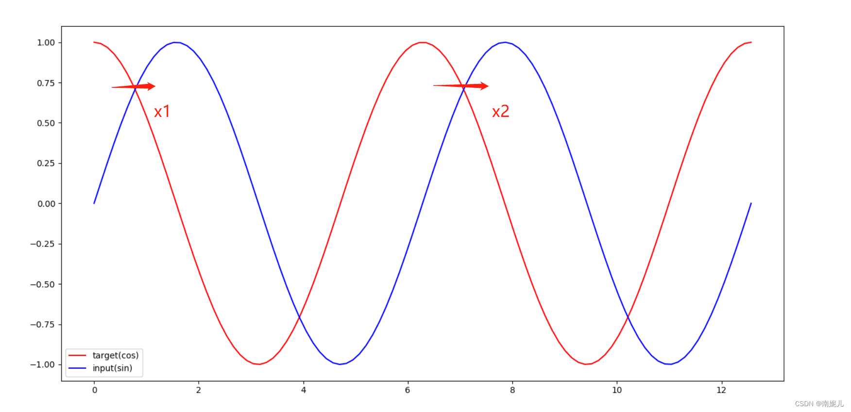
这里做一个预测问题,输入为sin值,输出对应的cos值。从上图中,可以看到x1和x2具有相同的cos值,但是对应的输入不一样,也就是说如果使用传统直连模型,这种预测问题是很不好做的。
import torch
from torch import nn

class Rnn(nn.Module):
    def __init__(self, input_size):
        super(Rnn, self).__init__()

        self.rnn = nn.RNN(
            input_size=input_size, ##输入特征的维度
            hidden_size=16,  ##隐藏层输出的维度
            num_layers=1,  ##隐藏层的个数
            batch_first=True
        )

        self.out = nn.Sequential(
            # nn.Linear(16,16),
            # nn.ReLU(),
            nn.Linear(160,1),
            # nn.Sigmoid()
        )

    def forward(self, x, h_state=None):
        r_out, h_state = self.rnn(x, h_state)
        out=self.out(r_out.flatten())

        return out, h_state

if __name__=='__main__':
    from torchinfo import summary
    model=Rnn(1)
    #输入  batchsize,seq_lenth,input_size
    input=torch.rand(1,10,1)
    summary(model)
    out,ht=model(input)
    print('预测的输出',out.shape)
    print('RNN最后一个时刻的输出',ht.shape)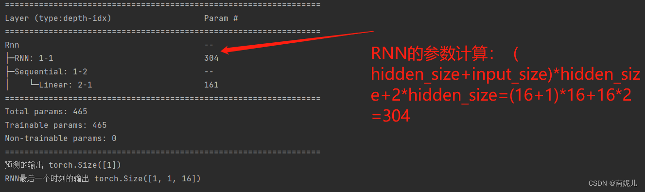
模型的训练
import numpy as np
import torch
from torch import nn
from models import Rnn

seq_lenth = 10  # 词向量的维度
input_size=1   #输入的维度

# 模型的模型的创建
model = Rnn(input_size)

# 定义优化器和损失函数
loss_func = nn.MSELoss()
optimizer = torch.optim.Adam(model.parameters(), lr=0.02)

h_state = None  # 第一次的时候,暂存为0

for epoch in range(10):
    epoch_loss=0
    for step in range(300):  ###生成3000个随机序列
        # 生成训练数据
        start, end = step , (step + 1)
        steps = np.linspace(start, end, seq_lenth, dtype=np.float32)
        x = torch.tensor(np.sin(steps))
        x = x.view(1, seq_lenth, 1)
        y = torch.tensor((np.cos(end)),dtype=torch.float32)
        y = y.view(1,1,1)

        prediction, h_state = model(x, h_state)
        # h_state = h_state.data
        h_state = h_state.detach()  # 隐藏层的状态不参与梯度传播

        loss = loss_func(prediction, y)
        epoch_loss=epoch_loss+loss.data
        optimizer.zero_grad()
        loss.backward()
        optimizer.step()
    print('第{}个epoch损失值'.format(epoch),epoch_loss/300)

torch.save(model,'./model{}.pth'.format(epoch)) 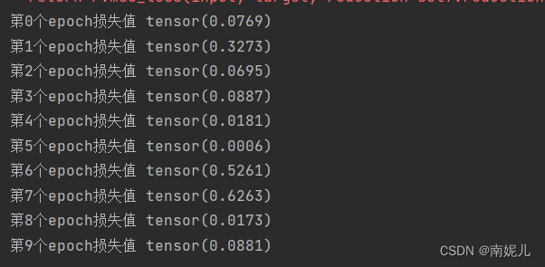
模型的测试
import numpy as np
import torch

import matplotlib.pyplot as plt
model=torch.load('model5.pth')
seg_lenth=10
h_state = None
x_true=[]
y_true=[]
y_predicted=[]
for step in range(300,350):  ###生成300个随机序列
    # 生成训练数据
    start, end = step , (step + 1)
    steps = np.linspace(start, end, seg_lenth, dtype=np.float32)
    x = torch.tensor(np.sin(steps))
    x_true.append((x[-1]))
    x = x.view(1, seg_lenth, 1)
    y = torch.tensor((np.cos(end)), dtype=torch.float32)
    y = y.view(1, 1, 1)
    y_true.append((y.data.numpy().flatten()))
    prediction, h_state = model(x, h_state)
    h_state = h_state.detach()
    y_predicted.append(prediction.data.numpy().flatten())

print('预测值',y_predicted)
print('真实值',y_true)
plt.plot(np.array(x_true),np.array(y_predicted), 'r-',label='predict')
plt.plot(np.array(x_true),np.array(y_true), 'b-',label='true')
# plt.plot(np.array(y_predicted),'r-',label='predict')
# plt.plot(np.array(y_true),'b-',label='true')
plt.legend(loc='best')
plt.show()

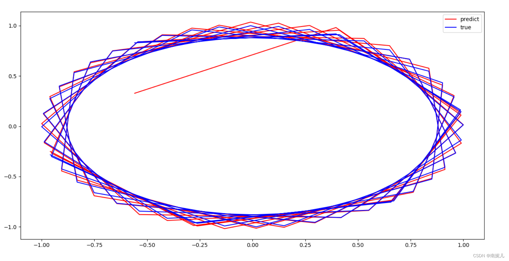
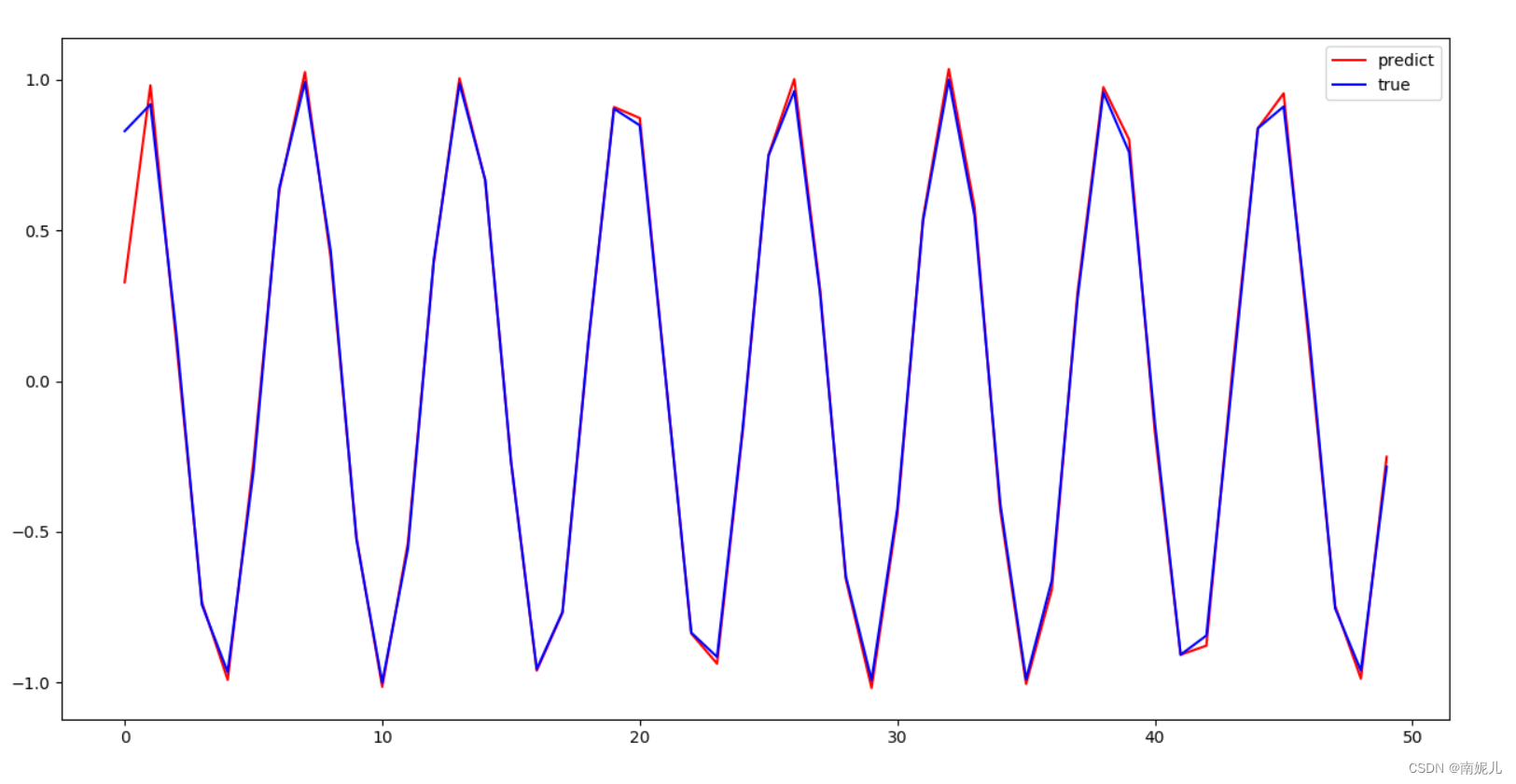
由上面的效果图,可以看到模型拟合的很好。但是最开始的值差别非常大。