目录
💥1 概述
📚2 运行结果
🎉3 参考文献
👨💻4 Matlab代码
💥1 概述
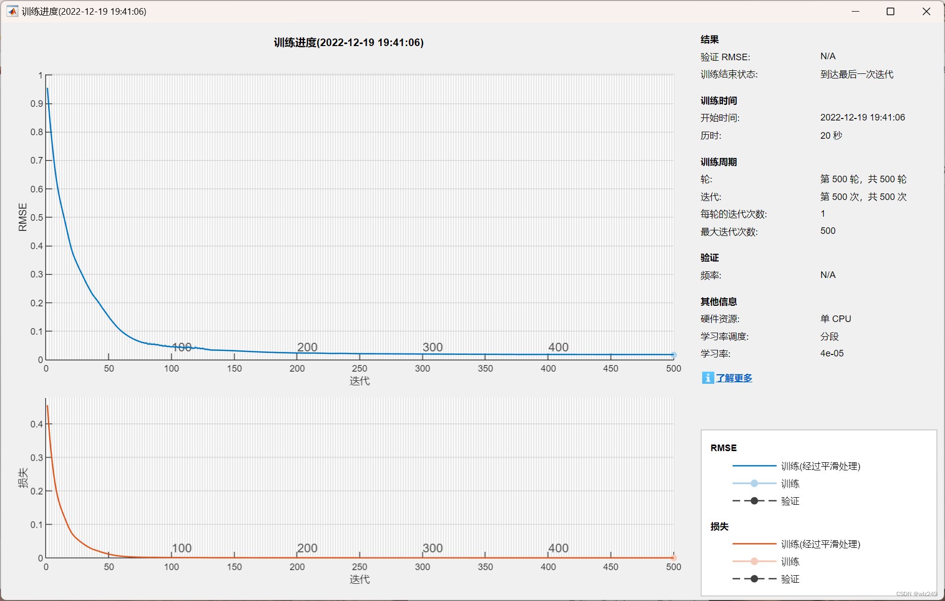
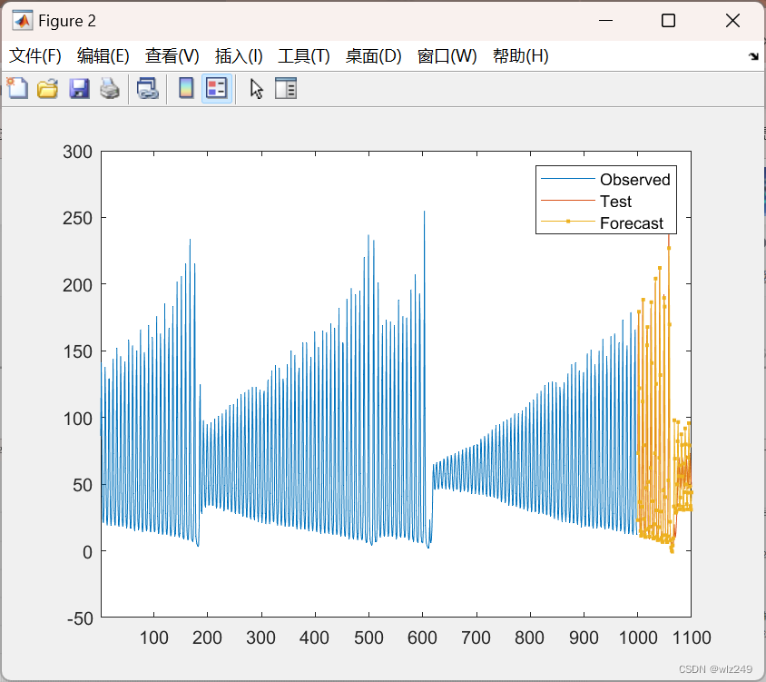
该项目为能源消耗的时间序列预测,在Matlab中实现。该预测采用多层人工神经网络,基于Kaggle训练集预测未来能源消耗。
📚2 运行结果
🎉3 参考文献
[1]程静,郑定成,吴继权.基于时间序列ARMA模型的广东省能源需求预测[J].能源工程,2010(01):1-5.DOI:10.16189/j.cnki.nygc.2010.01.012.
👨💻4 Matlab代码
seed = 52
rng(seed); % Seeds the random number generator using the nonnegative integer seed
% Load the data
load lasertrain.dat
load laserpred.dat
clear net
close all
p = 18; % Lag
n = 4; % Difference between the inputs and the number of neurons
[TrainData, TrainTarget] = getTimeSeriesTrainData(lasertrain, p); % This creates TrainData and TrainTarget, such as divided in time intervales of 5. TrainData(:,1) -> TrainTarget(1). R5 --> R1
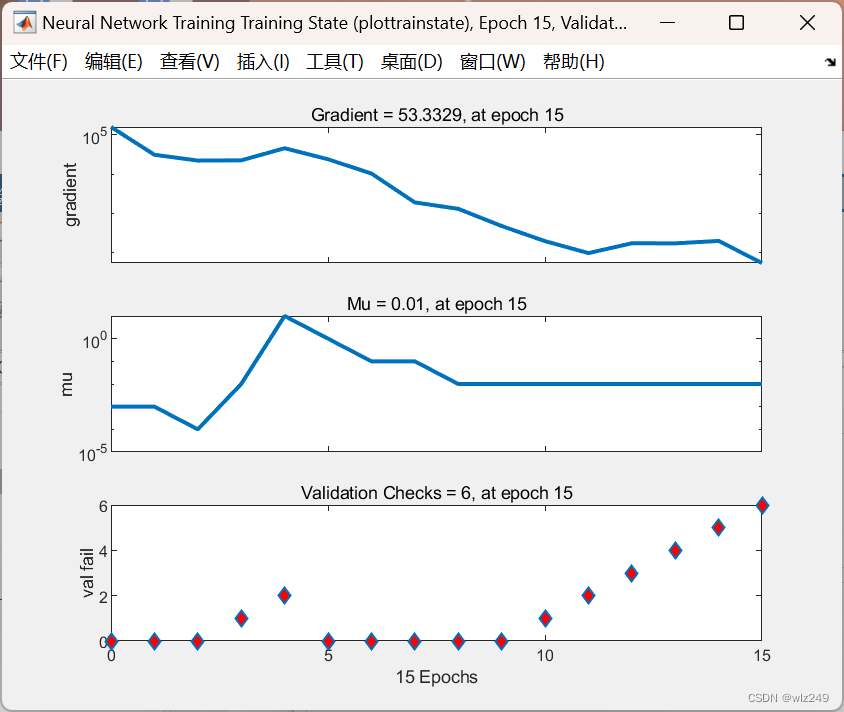
% Create the ANN
numN = p - n; % Number of neurons in the hidden layer
numE = 200; % Number of epochs
trainAlg = 'trainlm'; % Training Algorithm
transFun = 'tansig'; % Transfer Function
net = feedforwardnet(numN, trainAlg); % Create general feedforward netowrk
net.trainParam.epochs = numE; % Set the number of epochs for the training
net.layers{1}.transferFcn = transFun; % Set the Transfer Function
% net.divideParam.trainRatio = 0.8;
% net.divideParam.valRatio = 0.2;
% net.divideParam.testRatio = 0;
P = TrainData;
T = TrainTarget;
net = train(net,P,T);
TotMat = [lasertrain ; zeros(size(laserpred))];
for j = 1:length(laserpred)
r = length(lasertrain) - p + j;
P = TotMat(r:r+p-1);
a = sim(net,P);
TotMat(length(lasertrain) + j) = a;
% TotMat(length(lasertrain) + j) = (abs(round(a))+round(a))/2;
end
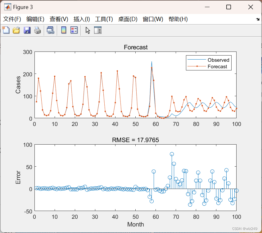
err = immse(TotMat(length(lasertrain)+1:end),laserpred);
x = linspace(1,length(TotMat),length(TotMat));
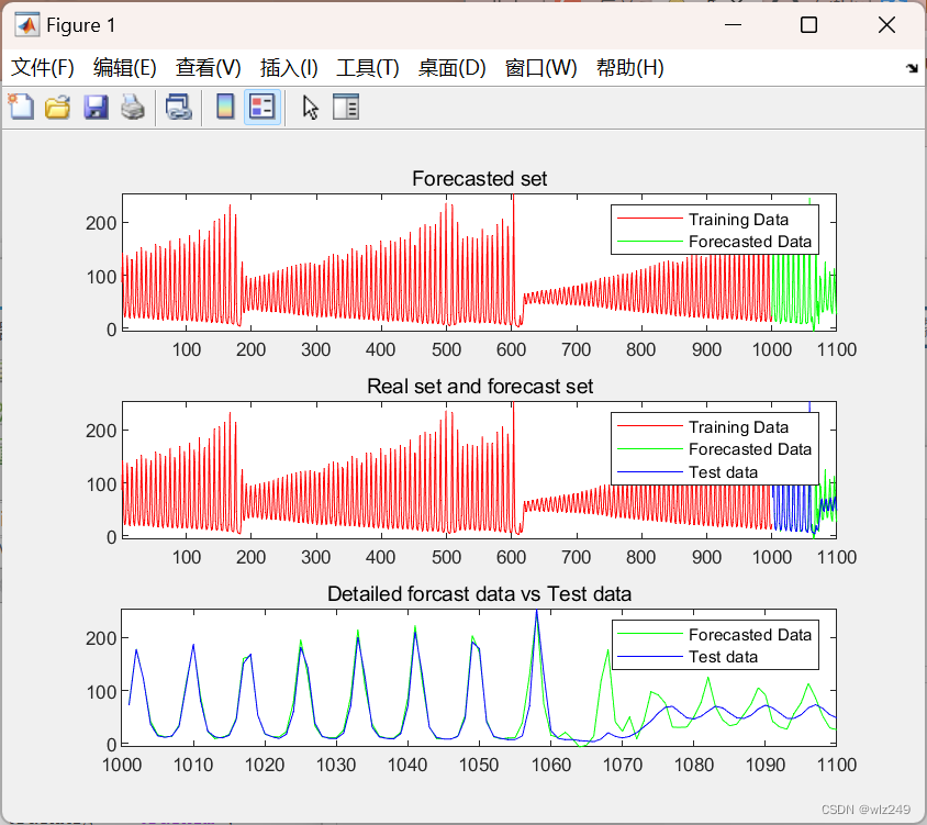
figure
subplot(3,1,2)
plot(x(1:length(lasertrain)), TotMat(1:length(lasertrain)),'r', x(length(lasertrain)+1:end), TotMat(length(lasertrain)+1:end),'g', x(length(lasertrain)+1:end), laserpred','b');
xlim([1 1100])
title('Real set and forecast set');
legend('Training Data','Forecasted Data', 'Test data');
subplot(3,1,1)
plot(x(1:length(lasertrain)), TotMat(1:length(lasertrain)),'r', x(length(lasertrain):end), TotMat(length(lasertrain):end),'g');
xlim([1 1100])
title('Forecasted set');
legend('Training Data','Forecasted Data');
subplot(3,1,3)
plot(x(length(lasertrain)+1:end), TotMat(length(lasertrain)+1:end),'g', x(length(lasertrain)+1:end), laserpred','b');
xlim([1000 1100])
title('Detailed forcast data vs Test data');
legend('Forecasted Data', 'Test data');
formatSpec = 'The mean squared error is %4.2f \n';
fprintf(formatSpec, err)
主函数部分代码:
%% Exercise 2 - Recurrent Neural Networks
%% Initial stuff
clc
clearvars
close all
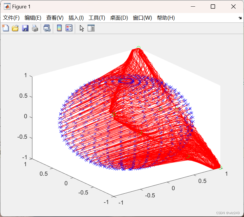
%% 1 - Hopfield Network
% Note: for this exercise, it will be interesting to check what happens if
% you add more neurons, i.e. modify T such as N is bigger.
T = [1 1; -1 -1; 1 -1]'; % N x Q matrix containing Q vectors with components equal to +- 1.
% 2-neuron network with 3 atactors
net = newhop(T); % Create a recurrent HOpfield network with stable points being the vectors from T
A1 = [0.3 0.6; -0.1 0.8; -1 0.5]'; % Example inputs
A2 = [-1 0.5 ; -0.5 0.1 ; -1 -1 ]';
A3 = [1 0.5 ; -0.3 -0.4 ; 0.8 -0.6]';
A4 = [0 -0.1 ; 0.1 0 ; -0.5 0.1]';
A5 = [0 0 ; 0 0.1 ; -0.1 0 ]';
A0 = [1 1; -1 -1; 1 -1]';
% Simulate a Hopfield network
% Y_1 = net([],[],Ai); % Single step iteration
num_step = 20; % Number of steps
Y_1 = net({num_step},{},A1); % Multiple step iteration
Y_2 = net({num_step},{},A2);
Y_3 = net({num_step},{},A3);
Y_4 = net({num_step},{},A4);
Y_5 = net({num_step},{},A5);
%% Now we try with 4 Neurons
T_ = [1 1 1 1; -1 -1 1 -1; 1 -1 1 1]'; % N x Q matrix containing Q vectors with components equal to +- 1.
% 4-neuron network with 3 atactors
net_ = newhop(T_); % Create a recurrent HOpfield network with stable points being the vectors from T
A1_ = [0.3 0.6 0.3 0.6; -0.1 0.8 -0.1 0.8; -1 0.5 -1 0.5]'; % Example inputs
A2_ = [-1 0.2 -1 0.2 ; -0.5 0.1 -0.5 0.1 ; -1 -1 -1 -1 ]';
A3_ = [1 0.5 1 0.5 ; -0.3 -0.4 -0.3 -0.4 ; 0.8 -0.6 0.8 -0.6]';
A4_ = [-0.5 -0.3 -0.5 -0.3 ; 0.1 0.8 0.1 0.8 ; -0.7 0.6 -0.7 0.6]';
% Simulate a Hopfield network
% Y_1 = net([],[],Ai); % Single step iteration
num_step_ = 40; % Number of steps
Y_1_ = net_({num_step_},{},A1_); % Multiple step iteration
Y_2_ = net_({num_step_},{},A2_);
Y_3_ = net_({num_step_},{},A3_);
Y_4_ = net_({num_step_},{},A4_);
%% Execute rep2.m || A script which generates n random initial points and visualises results of simulation of a 2d Hopfield network 'net'
% Note: The idea is to understand what is the relation between symmetry and
% attractors. It does not make sense that appears a fourth attractor when
% only 3 are in the Target T
close all